Using Python to extract ICESAT GLAS elevation data.

If you want to download and start using the code immediately, the code can be found at Github.

Background information

ICESat (Ice, Cloud,and land Elevation Satellite) is the benchmark Earth Observing System mission for measuring ice sheet mass balance, cloud and aerosol heights, as well as land topography and vegetation characteristics. From 2003 to 2009, the ICESat mission provided multi-year elevation data needed to determine ice sheet mass balance as well as cloud property information, especially for stratospheric clouds common over polar areas. It also provided topography and vegetation data around the globe, in addition to the polar-specific coverage over the Greenland and Antarctic ice sheets.

The ICESat collects elevation information using the GLAS (the Geoscience Laser Altimeter System). The GLAS includes a laser system to measure distance, a Global Positioning System (GPS) receiver, and a star-tracker attitude determination system.

The GLAH14 Dataset

The GLAH14 is the GLAS/ICEsat L2 Global Land Surface Altimetry Data (HDF5). For altimetry data on sea ice, ocean, or ice sheets, other data droducts are available.

The data is in HDF5 format (.H5). An HDF5 file is a container for two kinds of objects: datasets, which are array-like collections of data, and groups, which are folder-like containers that hold datasets and other groups. For the GLAH14 dataset, there is a detailed instruction on data structure and description. The GLAH14 data has rich information and to view the structures within the file, one easy way is to use the HDFView. It’s a free software that is available for most operation systems.

The workflow

Import necessary libraries

import pandas as pd
from shapely.geometry import Point
import h5py
from datetime import datetime, timedelta

Data extraction and transformation

Here I use pandas library for data ETL. Based on a simple benchmark test, using the pandas library for processing is a little bit faster than numpy in my case. It’s likely that someone who is more experienced in numpy can produce code of higher performance.

Like I mentioned, HDF5 file is hierarchical, and accessing the data is a lot like accessing files in nested folders:

with h5py.File(in_file_name, mode='r') as f:
    timestamp = f['/Data_40HZ/DS_UTCTime_40'][:]

The f['/Data_40HZ/DS_UTCTime_40'][:] is equivalent to f.groups['Data_40HZ'].variables['d_lat'][:]. You can easily see why I prefer the former syntax.

We can easily extract the record number, timestamp, longitude, and latitude information for each laser spot.

record_number = f['/Data_40HZ/Time/i_rec_ndx'][:]
timestamp = f['/Data_40HZ/DS_UTCTime_40'][:]

latvar = f['/Data_40HZ/Geolocation/d_lat']
latitude = latvar[:]

lonvar = f['/Data_40HZ/Geolocation/d_lon']
longitude = lonvar[:]

For elevation, it’s a bit tricky. Since the original data has varied level of quality, it’s important to filter out data that are noise. Also, GLAH14 has various types of correction that minimize the inaccuracy of elevation, these corrections need to be applied to achieve high level of data quality. A detailed list of definition of and how to use these corrections is available online.

elevar = f['/Data_40HZ/Elevation_Surfaces/d_elev']
elev = elevar[:]
elev_min, elev_max = int(elevar.attrs['valid_min']), int(elevar.attrs['valid_max'])

#satellite elevation correction
sat_ele_corr_var = f['/Data_40HZ/Elevation_Corrections/d_satElevCorr']
sat_ele_corr = sat_ele_corr_var[:]
sat_ele_corr_min, sat_ele_corr_max = int(sat_ele_corr_var.attrs['valid_min']), int(sat_ele_corr_var.attrs['valid_max'])

#elevation bias correction
ele_bias_corr_var = f['/Data_40HZ/Elevation_Corrections/d_ElevBiasCorr']
ele_bias_corr = ele_bias_corr_var[:]
ele_bias_corr_min, ele_bias_corr_max = int(ele_bias_corr_var.attrs['valid_min']), int(ele_bias_corr_var.attrs['valid_max'])
ele_bias_corr[ele_bias_corr < ele_bias_corr_min] = 0.0
ele_bias_corr[ele_bias_corr > ele_bias_corr_max] = 0.0

#satellite correction flag
sat_corr_flag = f['/Data_40HZ/Quality/sat_corr_flg'][:]

#elevation use flag
elev_use_flag = f['/Data_40HZ/Quality/elev_use_flg'][:]

Also, the height of the geoid above the ellipsoid, and the elevation at the footprint location from the SRTM30 (GTOPO30 + SRTM) Digital Elevation Model are available, too. This can be super convenient if you are doing change detection!

geoid = f['/Data_40HZ/Geophysical/d_gdHt'][:]

srtmvar = f['/Data_40HZ/Geophysical/d_DEM_elv']
srtm = srtmvar[:]
srtm_min, srtm_max = int(srtmvar.attrs['valid_min']), int(srtmvar.attrs['valid_max'])

The last step before exporting is to tabulate our data, and apply the filters and corrections to remove data of poor quality, and improve the accuracy.

columns=['RecordNumber', 'Timestamp', 'Latitude', 'Longitude', 
                    'Elevation', 'Sat_ele_corr', 'Ele_bias_corr', 'Sat_corr_flag',
                    'Elev_use_flag', 'Geoid', 'SRTM']
df = pd.DataFrame(dict(zip(columns, [record_number, timestamp, latitude, longitude, elev, sat_ele_corr, 
                                        ele_bias_corr, sat_corr_flag, elev_use_flag, geoid, srtm])))

df = df[(df['Latitude']<lat_max) & (df['Latitude']>lat_min)
    & (df['Longitude']<long_max) & (df['Longitude']>long_min) 
    & (df['Elevation']<elev_max) & (df['Elevation']>elev_min)
& (df['SRTM']<srtm_max) & (df['SRTM']>srtm_min)
    & (df['Sat_corr_flag']==2) & (df['Elev_use_flag']==0)]

df['Timestamp'] = base + pd.to_timedelta(df['Timestamp'], unit='s')
df['Timestamp'] = df['Timestamp'].values.astype('datetime64[s]')
df['Date'] = df['Timestamp'].dt.strftime('%Y/%m/%d')
df['Time'] = df['Timestamp'].dt.time.values.astype(str)
#converting the time to string otherwise Geopandas will raise error when exporting as .shp

df.loc[df['Longitude'] > 180, 'Longitude'] -= 360.0
#in the final output, the longitude will be converted to (-180, 180) instead of (0, 360).

df['Elevation_corrected'] = df['Elevation'] + df['Sat_ele_corr'] + df['Ele_bias_corr'] - df['Geoid'] - 0.7
df = df[['RecordNumber', 'Date', 'Time', 'Latitude', 'Longitude', 'Elevation_corrected', 'SRTM']]

Export data

Two options are available when exporting the data. The user can decide to either export the data in .csv format, or the .shp format if the user decides to use the output directly in a GIS environment.

if out_format == 'csv':
    df.to_csv(in_file_name.rsplit('.')[0] + '.csv')
else:
    geometry = [Point(xy) for xy in zip(df['Longitude'], df['Latitude'])]
    df = df.drop(['Longitude', 'Latitude'], axis=1)
    crs = {'init': 'epsg:4326'}
    gdf = gpd.GeoDataFrame(df, crs=crs, geometry=geometry)
    gdf.to_file(driver = 'ESRI Shapefile', filename= in_file_name.rsplit('.')[0] + '.shp')

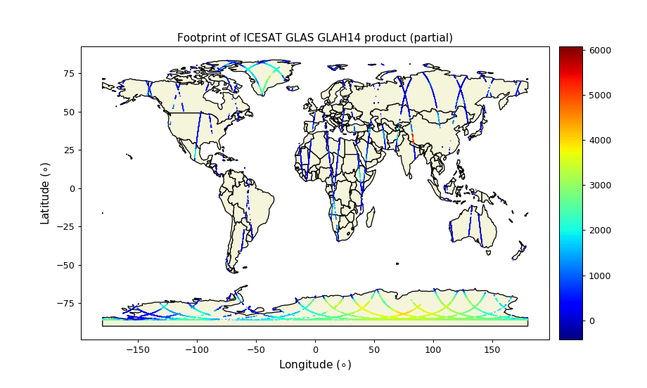
Mapping the laser footprints

We can map out the footprints of the dataset. The points are all over land mass (of course since we are using the LAND SURFACE Altimetry Data). The warmer color represents higher elevation and colder color represents lower elevation.

Trajectories of GLAS footprint